Running OpenQP from Python: Excited-State Analysis

Everything on the other pages can also be driven from Python. Python is the natural choice when the calculation is only the first step: here a script runs MRSF-TDDFT on formaldehyde and then analyses the excited states with natural transition orbitals (NTOs) and attachment/detachment densities, writing cube files for each.

S0→S1 hole NTO: the oxygen lone pair n

S0→S1 particle NTO: the C=O π*

Detachment density (0.004 a.u.): where the electron leaves

Attachment density (0.004 a.u.): where it arrives

The script

Download formaldehyde_analysis.py

"""MRSF-TDDFT of formaldehyde from Python, with NTO and attachment/detachment analysis."""
from oqp.openqp import OpenQP
from oqp.interop import MRSFExcitedStates, nto_transition, attachment_detachment
from oqp.export.cubegen import CubeExporter

job = OpenQP("formaldehyde_mrsf", silent=1)
job.molecule(
    """
C      0.000000     0.000000    -0.526342
O      0.000000     0.000000     0.676110
H      0.000000     0.937620    -1.119884
H      0.000000    -0.937620    -1.119884
""",
    charge=0,
)
job.theory.mrsf(functional="bhhlyp", basis="6-31g*", nstate=4)
mol = job.run()

results = mol.get_results()
ref = results["energy"]                # internal high-spin triplet reference
for n, de in enumerate(results["td_energies"]):   # state energies relative to it
    print(f"S{n}: {ref + de:.7f} hartree")

states = MRSFExcitedStates(mol)
cubes = CubeExporter(states)
for n in (1, 2):
    nto = nto_transition(states, 0, n)
    ad = attachment_detachment(states, n)
    print(f"S0 -> S{n}: oscillator strength {states.oscillator_strength(0, n):.4f}, "
          f"leading NTO weight {nto['weights'][0] / nto['weights'].sum():.3f}, "
          f"promoted electrons {ad['n_promoted']:.3f}")
    cubes.nto_cube(f"S{n}_hole.cube", nto["holes_ao"][:, 0], f"S{n} hole")
    cubes.nto_cube(f"S{n}_particle.cube", nto["particles_ao"][:, 0], f"S{n} particle")
    cubes.attachment_detachment_cubes(f"S{n}_attach.cube", f"S{n}_detach.cube", ad)

Run it with the Python environment in which OpenQP is installed:

python formaldehyde_analysis.py

• OpenQP(...), job.molecule(...), and job.theory.mrsf(...) set up the same calculation as the .oqp route mrsf(nstate=4)/bhhlyp/6-31g*; job.run() runs it and returns the molecule object with all results.
• results["energy"] is the energy of the internal high-spin triplet reference, and results["td_energies"] are the state energies relative to it; their sum is the absolute energy of each state.
• MRSFExcitedStates(mol) gives access to transition and difference densities. nto_transition(states, 0, n) computes the NTOs of the S0→Sn transition, attachment_detachment(states, n) the attachment and detachment densities.
• CubeExporter(states) writes Gaussian cube files on a regular grid for viewing in OQP Studio, VMD, or other programs.

The script takes about 20 seconds.

What you get

S0: -114.4212164 hartree
S1: -114.2710381 hartree
S2: -114.1004661 hartree
S3: -114.0941225 hartree
S0 -> S1: oscillator strength 0.0000, leading NTO weight 1.000, promoted electrons 1.043
S0 -> S2: oscillator strength 0.0052, leading NTO weight 1.000, promoted electrons 1.104

and eight cube files, S1_hole.cube to S2_detach.cube. The S1 energy agrees with the .oqp runs at this geometry (4.087 eV above S0).

Reading the result

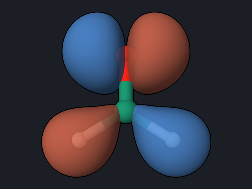
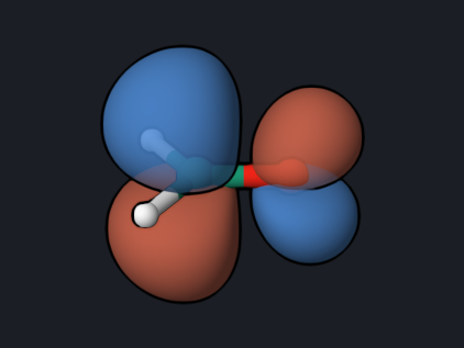
• One NTO pair describes S1 completely. The leading NTO weight is 1.000: S0→S1 is a single, clean excitation from the oxygen lone pair n into the C=O π* orbital, as the pictures show.
• About one electron is promoted. The promotion number 1.04 counts how many electrons move between the detachment and attachment densities; a value near 1 is what a single excitation gives.
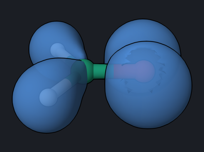
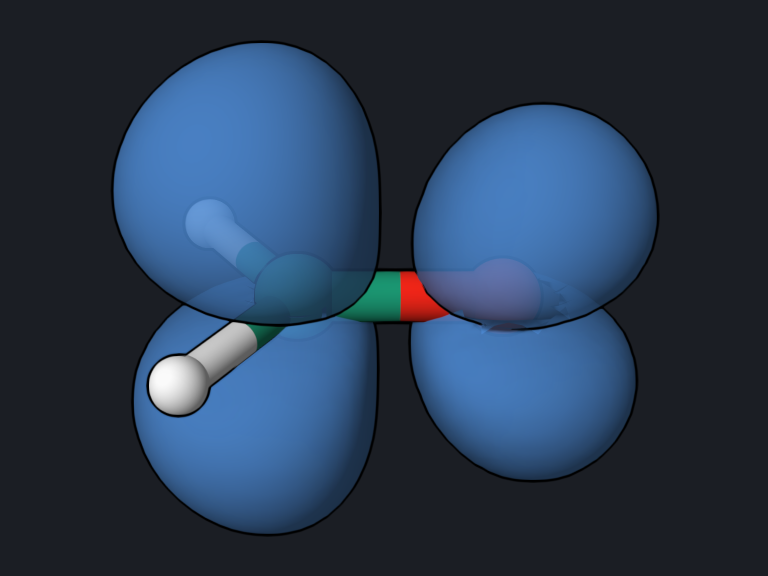
• Attachment and detachment show the same n→π* change as density differences: the electron leaves the in-plane lone-pair region on oxygen and arrives in the π* lobes above and below the C=O bond.

Try next

• Analyse S0→S2 in the same way and open S2_hole.cube and S2_particle.cube.
• Pass a fragment list to analyze_mrsf_transition (see MRSF Analysis and Interoperability) to split a larger molecule into donor and acceptor parts and measure charge-transfer character.

See also: Run OpenQP from Python, MRSF Analysis and Interoperability, Python API.

Scientific references

Excited-state analysis and ionization.