Ethylene: Nonadiabatic Dynamics from S1

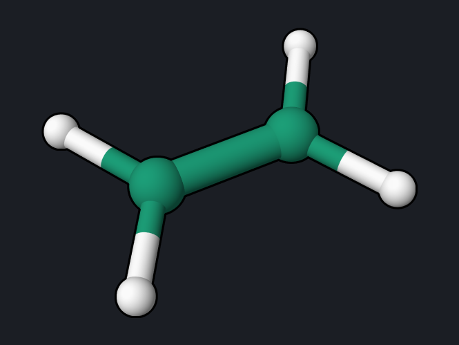
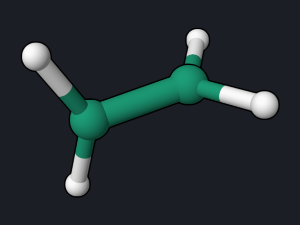
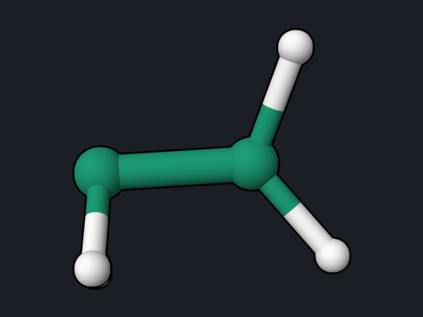
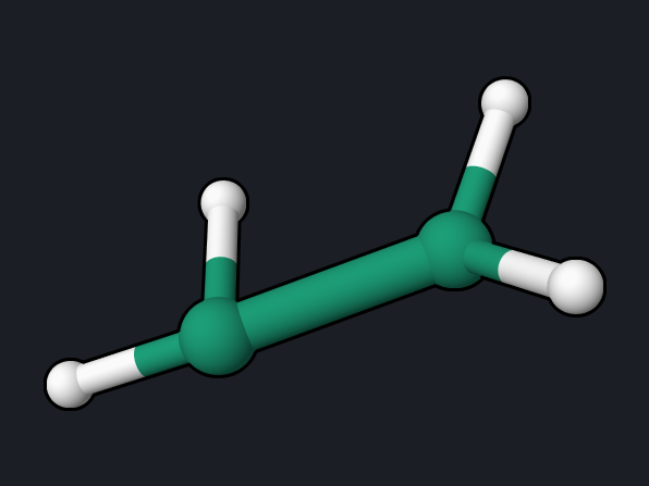
Surface-hopping molecular dynamics follows the nuclei classically on one electronic state at a time and lets them hop between states. This example starts one trajectory of ethylene on S1 and follows it for 150 fs: the C=C bond twists, the molecule reaches the region of the conical intersection, and it returns to S0.

t = 0 fs, planar, on S1

t = 25 fs, twisted

t = 101.5 fs, hop to S0

t = 123 fs, vibrationally hot S0

Copy and run

ethylene-namd.oqp

mrsf(nstate=3)/bhhlyp/6-31g namd(S1,scheme=BaeckAn) md(nstep=300,dt=0.5,temperature=300,seed=7)
geom="""
C      0.000000     0.000000     0.664311
C      0.000000     0.000000    -0.664311
H      0.000000     0.923944     1.237411
H      0.000000    -0.923944     1.237411
H      0.000000     0.923944    -1.237411
H      0.000000    -0.923944    -1.237411
"""

Download ethylene-namd.oqp

openqp ethylene-namd.oqp

• mrsf(nstate=3)/bhhlyp/6-31g: three MRSF-TDDFT singlet states. The smaller 6-31G basis set keeps each step to about 2 seconds.
• namd(S1,scheme=BaeckAn): start on S1 and use Tully surface hopping with Baeck–An time-derivative couplings, which are computed from the state energies alone.
• md(nstep=300,dt=0.5,temperature=300,seed=7): 300 steps of 0.5 fs, initial velocities drawn from a 300 K Maxwell–Boltzmann distribution with a fixed random seed, so the run is reproducible.

The run takes about 9 minutes with 4 threads.

What you get

Each step prints one line to the log; active is the current state (1 = S0, 2 = S1, 3 = S2) and pop the electronic populations:

   NAMD step    202  t=  101.000 fs  active=2  E_tot=-78.19130471  E_pot=-78.26615272 ...
   NAMD step    203  t=  101.500 fs  active=1  E_tot=-78.19055127  E_pot=-78.28035803 ...

The full trajectory, with all state energies, populations, couplings, coordinates, and velocities at every step, is in the binary file ethylene-namd.namd.trj. Read it from Python:

from oqp.library.namd import read_namd_trajectory

header, rec = read_namd_trajectory("ethylene-namd.namd.trj")
t = rec["time_fs"]                 # (nstep,)
energies = rec["state_energies"]   # (nstep, nstate) in hartree
active = rec["active"]             # 1-based active state
xyz = rec["coordinates_bohr"]      # (nstep, natom, 3)

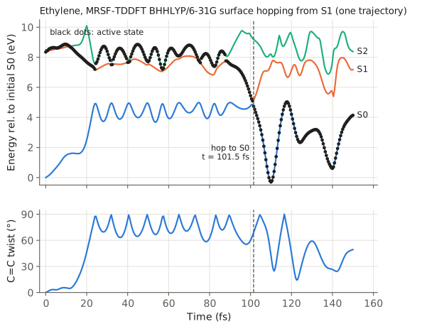
Event	Reference trajectory
Initial kinetic temperature	395 K (one random sample of the 300 K distribution)
C=C twist reaches about 90°	by 25 fs
Hops between S1 and S2	10, between 1.5 and 88 fs
Hop to S0	101.5 fs, where the S1–S0 gap is 0.23 eV
Total-energy range over 150 fs	2.0 × 10⁻³ hartree (0.05 eV)

The static picture: S1 minimum-energy path

The trajectory follows the steepest way down on S1 only roughly, because the nuclei carry kinetic energy. The minimum-energy path (MEP) on S1 from the Franck–Condon region shows the underlying landscape:

ethylene-s1-mep.oqp

mrsf(nstate=5)/bhhlyp/6-31g* mep(S1,maxit=100)
geom="""
C      0.000000     0.000000     0.664311
C      0.000000     0.000000    -0.664311
H      0.000000     0.923944     1.237411
H      0.000000    -0.923944     1.237411
H     -0.080527     0.920428    -1.237411
H      0.080527    -0.920428    -1.237411
"""

Download ethylene-s1-mep.oqp

The start is the planar geometry with one CH₂ group turned by 5°: at an exactly planar structure the S1 gradient has no twisting component, and the path would only stretch the C=C bond. mep(S1) then steps downhill on S1 until it reaches a minimum (about 4.5 minutes):

   PyOQP: MEP Bracketed A Minimum Basin (30 points)

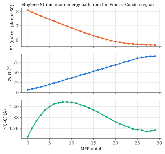
Along the path S1 falls from 8.09 eV to 5.66 eV (relative to the planar S0 minimum) while the twist grows from 7° to 90°; r(C–C) stays near 1.35 Å. The S1 minimum is the 90° twisted structure, the same region the trajectory reaches within 25 fs (the path uses 6-31G*, the trajectory the smaller 6-31G basis set). The geometries of all points are in mep_geom.xyz.

Reading the result

• S1 and S2 are nearly degenerate at the start (8.38 and 8.42 eV at the planar geometry, see the twist example), so the trajectory hops between them several times in the first 90 fs.
• Twisting is fast. Within 25 fs the CH₂ planes are almost perpendicular and the S1–S0 gap has fallen from 8.4 eV to about 2.4 eV.
• Return to S0 happens at 101.5 fs, at a twist of 69°, close to the 70° twist of the MECI. After the hop the released electronic energy becomes vibration: toward the end of the run the C–H bonds stretch up to 1.42 Å (1.09 Å at the start).
• One trajectory is not a result. Lifetimes and quantum yields need an ensemble of trajectories from sampled initial conditions; see the md keyword pages.

Try next

• Change seed=7 to other values to run more trajectories; each one follows a different path.
• Use 6-31g* for a more accurate surface; each step then takes longer.

See also: md keywords, NAMD coupling schemes, NAMD diagnostics.

Scientific references

Nonadiabatic Dynamics; MRSF-TDDFT.