Ethylene with CASSCF and XMCQDPT2
The twist example treats twisted ethylene with MRSF-TDDFT. This page uses wavefunction methods for the same problem: CASSCF geometry optimizations of planar and twisted ethylene with two electrons in the π and π* orbitals, and multistate perturbation theory (XMCQDPT2) for the ground and excited states.
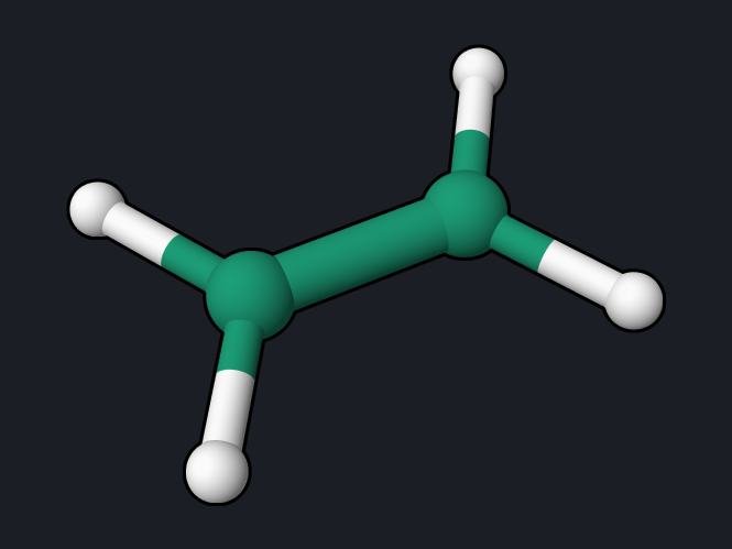
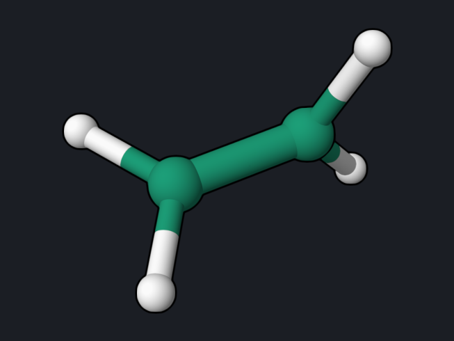
Step 1: CASSCF(2,2) geometry optimization
casscf/6-31g* opt cas(active_electrons=2,active_orbitals=2)
geom="""
C      0.000000     0.000000     0.664311
C      0.000000     0.000000    -0.664311
H      0.000000     0.923944     1.237411
H      0.000000    -0.923944     1.237411
H      0.923944     0.000000    -1.237411
H     -0.923944     0.000000    -1.237411
"""
Download ethylene-twisted-casscf-opt.oqp · ethylene-planar-casscf-opt.oqp (same first line, planar start)
CASSCF optimizes the orbitals and the configuration-interaction coefficients
together, and OpenQP computes its nuclear gradient analytically, so opt works
directly. The twisted start keeps its D2d symmetry, so the optimization finds
the best twisted structure, which is the transition state for rotation about
the C=C bond. The two runs take 7 and 11 seconds.
| Structure | E(CASSCF) (hartree) | r(C–C) | r(C–H) | ∠HCH |
|---|---|---|---|---|
| Planar minimum | −78.0602554 | 1.338 Å | 1.076 Å | 116.5° |
| Twisted (90°), optimized | −77.9580116 | 1.465 Å | 1.076 Å | 117.2° |
The relaxed rotation barrier is 0.1022 hartree, 2.78 eV (64 kcal/mol), close to the experimental activation energy for cis–trans isomerization of ethylene derivatives of about 65 kcal/mol. With bond lengths frozen at the planar values the barrier is 3.20 eV (the dashed curve on the twist page): stretching the C–C bond to 1.465 Å, close to a single bond, lowers the twisted structure by 0.4 eV.
Step 2: XMCQDPT2 for the ground and excited states
xmcqdpt2/6-31g* cas(active_electrons=2,active_orbitals=2,frozen_core=7) ci(nroot=3,target_spin=singlet) pt2(target_roots="0,1,2",nroot=3,edshft=0.02)
geom="""
C      0.000000     0.000000     0.664311
C      0.000000     0.000000    -0.664311
H      0.000000     0.923944     1.237411
H      0.000000    -0.923944     1.237411
H      0.000000     0.923944    -1.237411
H      0.000000    -0.923944    -1.237411
"""
Download ethylene-planar-xmcqdpt2.oqp · ethylene-twisted-xmcqdpt2.oqp (the 90° geometry)
xmcqdpt2is extended multiconfiguration quasi-degenerate second-order perturbation theory: three CAS(2,2) states are corrected together and allowed to mix, which keeps the states smooth near degeneracies.frozen_core=7counts the seven doubly occupied orbitals outside the active space (see the LiH page for this convention), andedshft=0.02is a small denominator shift that avoids intruder states.
Each run takes about 4 seconds. The geometries are those of the MRSF twist scan, so the results can be compared directly:
| Quantity | XMCQDPT2 | MRSF-TDDFT | CASSCF(2,2) |
|---|---|---|---|
| S0 rise at 90° (rigid twist) | 3.17 eV | 3.54 eV | 3.20 eV |
| S0 → S1 at the planar geometry | 8.80 eV | 8.38 eV | — |
| S1 − S0 at 90° | 2.68 eV | 2.23 eV | — |
   PyOQP state 0                            -78.2943723081
   PyOQP state 1                            -77.9710533525
   PyOQP state 2                            -77.7803082396
Reading the result
- CASSCF(2,2) gets the shape right at very low cost: it is the minimal wavefunction that describes the broken π bond at 90°. Its rotation barrier is close to experiment.
- The excitation energies need dynamic correlation. The planar S1 (the ππ* V state) is notoriously sensitive to σ–π correlation; with a CAS(2,2) reference and the 6-31G* basis set XMCQDPT2 puts it at 8.80 eV, and MRSF-TDDFT at 8.38 eV, both above the experimental band maximum of about 7.7 eV. A larger active space and diffuse basis functions are needed for a quantitative V state.
- For the ground-state twist barrier, the three methods agree within 0.4 eV.
Try next
- Use
xms-caspt2instead ofxmcqdpt2for a small molecule (see the LiH page for the size limit of the uncontracted CASPT2). - Optimize the excited state with
casscf/6-31g* opt(S1)and state averaging, as in the repositoryexamples/WF_methods.
See also: CASSCF Nuclear Gradient, Wavefunction methods.